Motivation: Due to the significantly increased computational cost of simulating fluids with Pr > 1, in practice numerical simulations of turbulent wakes in water are performed using Pr=1 despite the fact that Pr=7 for thermally stratified water and Pr~700 for salt and thermally stratified water in the ocean. This assumes that the Prandtl number has a very small impact on the flow. Is this assumption reasonable? How does the Prandtl number affect the wake in a stratified fluid?
Direct numerical simulation was used to study the effect of Pr on a turbulent stratified wake at Re=10,000. Three values of Pr were simulated: Pr = 0.2, 1, and 7. To give an idea of the different computational cost required at different values of Pr, the Pr=0.2 and Pr=1 cases required 168 million grid points and 800 CPU hours on 40 processors. The Pr=7 case required 1.88 billion grid points and 14,000 CPU hours on 448 processors. The simulations were run from 6 body diameters to 1,200 body diameters downstream of the body; a range that encompasses the near, intermediate and far wake. Bulk quantities such as wake defect velocity and the wake dimensions were found to be weakly influenced by the Prandtl number. However, the Prandtl number was found to strongly affect the density perturbation field. Through the coupling between kinetic and potential energy, differences in the density perturbation field resulted in differences in the wave flux, total energy of the wake, turbulent and scalar dissipation, spectral distribution of energy in the density and velocity fields, mixing efficiency, and buoyancy flux.
Important conclusion: For 0.2 < Pr < 7 the qualitative behavior of the wake is the same as Pr=1. There are differences in a number of small scale features but these changes are small relative to the significantly higher computational cost.
For further details on this work, see the 2010 Physics of Fluids paper by de Stadler, Sarkar, and Brucker. pdf
 |
 |
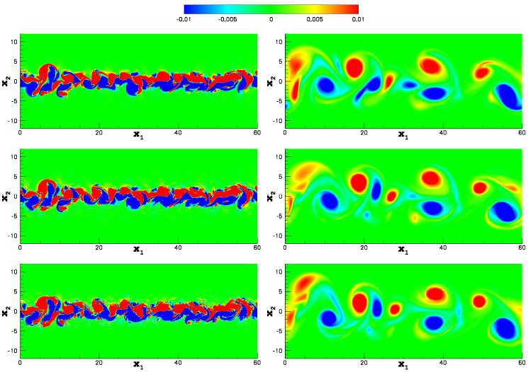 |
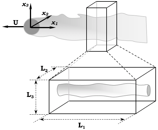
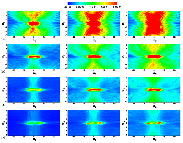
| Simulation setup. Simulations are performed in the temporally evolving frame shown at the bottom. | Density perturbation field as a function of time. (Left column) Pr=0.2, (Middle column) Pr=1 (Right column (Pr=7). The top row is at the earliest time and the bottom row the latest. Differences in the density field are one of the most significant changes that occur at different values of Pr. | Vorticity field, &omega3, at the horizontal centerplane x3=0 (looking down at the wake from above). (Left column) t = 100. (Right column) t=1200. (Top) Pr=0.2. (Middle) Pr=1. (Bottom) Pr=7. Note the similarities between the three cases at both times. |
| Movie showing the evolution of the mean streamwise velocity in the wake. Note the asymmetry due to stratification. | Movie showing the density perturbation as the wake evolves. The density perturbation is one way of visualizing internal waves. | Movie showing the vorticity, &omega3, at the horizontal centerplane, x3=0. Note the large pancake vortices formed in the late wake. |