Motivation: Develop familiarity with a simple stratified turbulent flow and performing numerical simulations.
When I first got to graduate school I began to perform simulations of a stratified shear layer. A shear layer occurs when a flow transitions from one
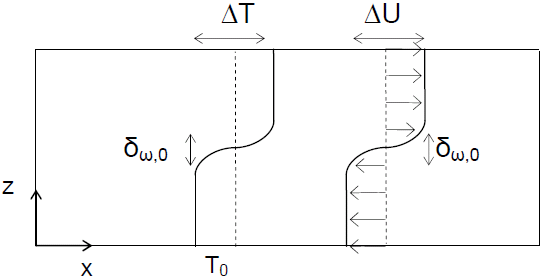
velocity to another over a relatively short distance in the transverse direction (illustrated in the figure below). For analytical and numerical
convenience the mean streamwise velocity is
often subtracted off the streamwise flow profile so that the flow transition from U=-ΔU/2 to U=+ΔU/2 where ΔU is the velocity difference
between the flow in the two regions.
Shear layers are good test problems for turbulent codes because they are the simplest possible turbulent free shear flow problem. Variations are
initially present in only one dimension and periodic boundary conditions can be used in the other two dimensions. There is a strong production of
turbulence from the background flow which makes the problem less sensitive to initial conditions than other similar problems such as jets and wakes.
Another benefit is that results from
the fully turbulent case agree reasonably well with predictions from linear stability theory, at
least in regards to the wavelength of the fastest growing mode and the length scale governing the number of and spacing between Kelvin-Helmholtz rollers.
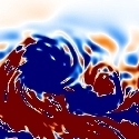
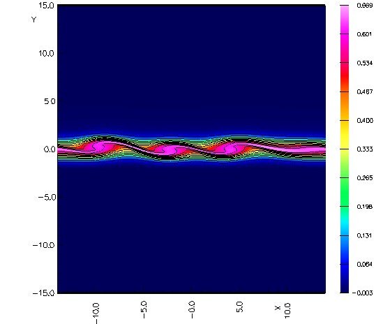
The tendency of the fluid interface to roll up and form Kelvin-Holmholtz rollers is a well known result of shear instability.
The destabilizing impact of shear can be compared with the stabilizing impact of viscosity by performing simulations at different Reynolds numbers.
The stabilizing impact of buoyancy can be seen in that significantly different results are observed at different values of the bulk Richardson
number with linear stability theory predicting that
a necessary condition for instability is that somewhere in the flow, Rib < 0.25. While the initial instability is strongly two-dimensional
in nature, once perturbations reach finite amplitude secondary instabilities with a more three-dimensional character form. In general results from
2D simulations tend to look 'cleaner' than equivalent 3D simulations.
Unstratified 2D shear layer report
Report comparing 2D shear layer simulations with linear stability theory
 |
 |
| Shear layer problem formulation. Two parallel streams of fluid with equal magnitude but opposite sign values. The small transition region in the center of the domain where the flow goes from -U to +U is referred to as a shear layer. | Vorticity field from a 2D simulation with Re=600 and Ri=0.05 showing the formation of Kelvin-Helmholtz rollers. |
|
Movie showing the vorticity field for a stratified 2D simulation at Re=600, Ri=0.05 |
Movie showing the temperature field for a stratified 2D simulation at Re=600, Ri=0.05 |
Movie showing the vorticity field for an unstratified 2D simulation at Re=2,000 |